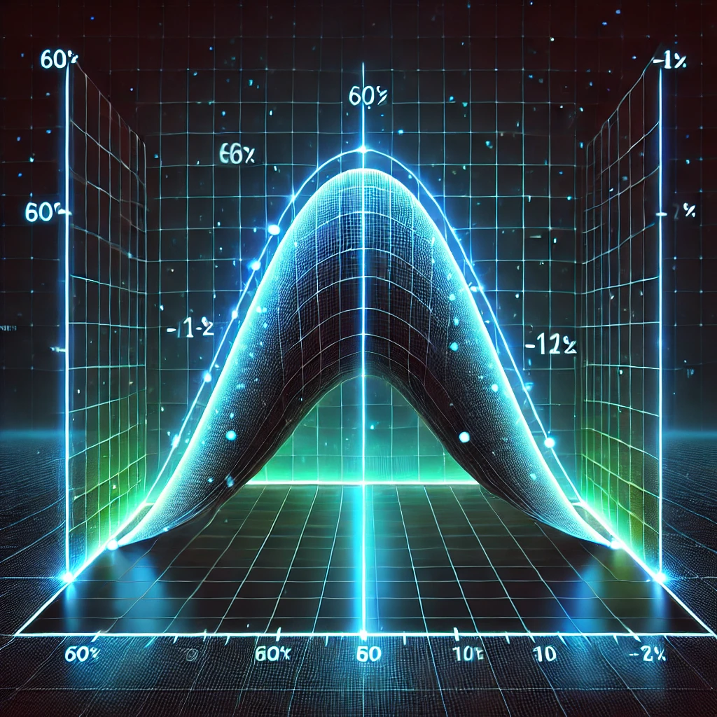
Monte Carlo analysis is one of the most powerful techniques available when working with uSimmics (formerly QucsStudio). It lets you quantitatively assess how manufacturing tolerances and environmental variation affect circuit performance. This article focuses specifically on the tol function used in Monte Carlo analysis — covering its syntax, the meaning of each argument, the differences between distribution types, and key pitfalls to avoid.
What You’ll Learn
- The fundamentals of Monte Carlo simulation and its role in circuit design
- The syntax and argument meanings of the
tolfunction in uSimmics (formerly QucsStudio) - The difference between normal (Gaussian) and uniform distributions, and when to use each
- How to correctly model component manufacturing tolerances with the tol function
- How to avoid simulation errors caused by misconfigured parameters
What Is Monte Carlo Simulation?
Monte Carlo simulation is a probabilistic method for evaluating systems and processes that involve uncertainty. By assigning random values to input variables and repeating the calculation many times, it produces a statistical picture of how the system behaves across its expected operating range.
In circuit design, a typical use case is this: if resistors and capacitors have a ±5% manufacturing spread, how does that spread propagate into the overall circuit’s performance — cutoff frequency, gain, phase margin, and so on? Monte Carlo simulation answers that question statistically.
The tol function deserves dedicated attention because a large number of users are unsure how to specify component variation correctly, and misconfigured parameters frequently lead to simulation results that diverge significantly from reality.
Modeling Component Variation
Before running a Monte Carlo simulation, you need to define both the variation range and the distribution type for each input variable. uSimmics (formerly QucsStudio) provides the tol function as a concise way to do this.
With tol, you define how much a particular component value (resistance, capacitance, etc.) varies around its nominal value, directly embedding manufacturing tolerances and environmental effects into the simulation.
tol Function Syntax and Arguments
The tol function in uSimmics (formerly QucsStudio) takes the following form:
tol(x, v, d)
| Argument | Meaning | Example |
|---|---|---|
x |
Nominal (mean) value | 100 (100 Ω) |
v |
Tolerance range (%) | 10 (±10%) |
d |
Distribution type (0 = normal, 1 = uniform; default is 0) |
0 |
Example: 100 Ω Resistor with ±10% Tolerance
To model a resistor with a nominal value of 100 Ω and a ±10% tolerance:
tol(100, 10, 0)
100— nominal (center) value10— tolerance range (±10%)0— normal (Gaussian) distribution
Distribution Types in Detail
The third argument, the distribution type, directly affects the validity of your simulation results. It is important to understand the characteristics of each distribution and choose appropriately.
Normal (Gaussian) Distribution: d=0
Values are symmetrically distributed around the mean. The farther a value is from the mean, the less likely it is to occur. The shape is a bell curve.
An important caution on setup:
When v is set to ±10%, the standard deviation (σ) is set to 10% (i.e., 10 Ω). Because a normal distribution theoretically extends to ±∞, a portion of sampled values will fall outside the 90–110 Ω range. In other words, values beyond the stated ±10% tolerance will appear in the simulation. This can create a significant and misleading discrepancy when the goal is to model real component variation accurately.
Uniform Distribution: d=1
Values are distributed evenly across the specified range, with every value within that range equally likely to occur. The shape is flat (rectangular).
When v is set to 10%, values are spread uniformly between 90 Ω and 110 Ω; no values fall outside that range. The upper and lower bounds are strictly ±10%.
That said, real electronic components actually follow a normal distribution — values near the nominal are more common, and values near the tolerance limits are increasingly rare. A uniform distribution therefore does not accurately represent the spread of real components.
Choosing Between Distribution Types
| Distribution Type | Characteristics | Recommended Use |
|---|---|---|
| Normal (d=0) | Concentrated near the mean; tails extend beyond the tolerance | Closest to real component behavior, but requires careful standard deviation setup |
| Uniform (d=1) | Equal probability within the range; zero probability outside | Worst-case analysis, safety-margin studies |
A Critical Note: Manufacturing Tolerance vs. Standard Deviation
Real resistors and capacitors follow a normal distribution, but the tolerance figures (e.g., ±5%) quoted in component datasheets are typically set by manufacturers to correspond to 3σ (three standard deviations) of the production distribution.
Plugging the datasheet tolerance percentage directly into the v argument of tol will therefore run the simulation with three times the actual component variation. For guidance on how to calculate the correct standard deviation and enter it into tol, see the related article on standard deviation parameter configuration for real components.
Summary
Configuring the tol function correctly is essential for accurately modeling random variation in Monte Carlo simulation. Understand the characteristics of normal and uniform distributions and select the type that matches your simulation objective. When using a normal distribution in particular, always verify that the standard deviation value you enter corresponds to the actual manufacturing tolerance specification — otherwise, your results may significantly overstate the circuit’s sensitivity to component variation.
Related Articles
- uSimmics (formerly QucsStudio) Monte Carlo Analysis: Setting Standard Deviation Parameters for Real Components [2026]
- Parametric Analysis of Electronic Circuits with uSimmics (formerly QucsStudio) [2026]
- uSimmics (formerly QucsStudio) vs. QUCS: Key Differences and Evolution [2026]
- How to Change the Project Folder Location in uSimmics (formerly QucsStudio) [2026]
- Low-Pass Filter Design Fundamentals and Simulation

Comment