uSimmics (formerly QucsStudio) includes a Power Matching feature that significantly speeds up RF system design. This article walks through the complete workflow for automatically generating an impedance matching network from an antenna S-parameter file — from file import through simulation verification.
What You’ll Learn
- What the Power Matching feature in uSimmics (formerly QucsStudio) does and when to use it
- How to import an S-parameter file into uSimmics (formerly QucsStudio)
- How to place frequency markers and auto-generate a matching circuit
- How to verify the generated matching network through simulation
- When to use automatic matching versus manual Smith-chart-based design
1. What Is Impedance Matching?
Impedance matching is the practice of aligning the impedances of a source, transmission line, and load so that maximum power is transferred with minimal reflection. In RF systems, 50 Ω is the standard reference impedance, and components such as antennas and filters must be matched to this value.
When an impedance mismatch exists, the following problems arise:
- Signal reflections cause power loss (quantified by the reflection coefficient Γ)
- Amplifier output power decreases
- Receiver sensitivity degrades
- Unwanted radiation increases
Manual matching design requires iterative Smith chart calculations. The Power Matching feature in uSimmics (formerly QucsStudio) automates this process entirely.
2. Components and Files Used
This article uses the Wi-Fi antenna 2450AD14A5500 as a practical example. S-parameter files for this antenna (Touchstone format: .s1p or .s2p) are publicly available, making it a convenient real-world test case.
The antenna is optimized for the 2.4 GHz and 5 GHz bands. The target for this exercise is matching to 50 Ω at 5800 MHz.
3. Step-by-Step Automatic Matching Procedure
Step 1: Create a New Project and Build the Schematic
- Launch uSimmics (formerly QucsStudio).
- Create a new project from the menu.
- Place an S-parameter file component (SPfile) from the component library onto the schematic.
- Load the antenna S-parameter file (
.s1p) into the component. - Connect a Port component to define the simulation termination.
Step 2: Configure the S-Parameter Simulation
- From the Simulations tab, place an S-Parameter Simulation component.
- Set the frequency sweep range (for example, 2 GHz to 6 GHz in 10 MHz steps).
- Confirm that the sweep covers both the 2.4 GHz and 5 GHz antenna operating bands.
Step 3: Run the Initial Simulation and Review Results
- Click the simulate button to run the S-parameter calculation.
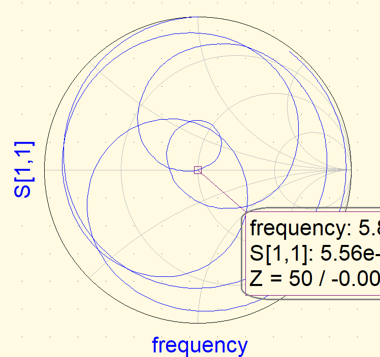
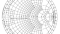
- After simulation completes, display S11 (return loss) on a Smith chart or rectangular plot in the graph window.
- Inspect the antenna impedance characteristic. At 5800 MHz the impedance is likely to deviate from 50 Ω, confirming that a matching network is needed.
Step 4: Place a Marker and Run Power Matching
The Marker feature captures the impedance at a specific frequency, which is then fed directly into the automatic matching generator.
- Right-click on the graph and select Add Marker.
- Place the marker at 5800 MHz.
- Right-click the marker and select Power Matching from the context menu.
- In the Power Matching dialog, configure the following parameters:
- Reference impedance: 50 Ω
- Matching network topology (LC ladder, π-network, etc.)
- Component types (inductors and capacitors)
- Click Create to auto-generate the matching circuit.
Step 5: Connect the Matching Circuit and Re-simulate
- The generated matching circuit appears on the schematic.
- Connect it to the antenna port.
- Run the simulation again.
- Verify that the S11 at 5800 MHz has improved (target: −20 dB or better).
- Confirm on the Smith chart that the 5800 MHz impedance has converged to the center (50 Ω).
After matching, the simulation results should show a substantial reduction in return loss at 5800 MHz, confirming that the 50 Ω optimization target has been met.
4. Automatic Matching vs. Manual Matching: Choosing the Right Approach
| Criterion | Power Matching (automatic) | Manual Matching |
|---|---|---|
| Design speed | Fast (seconds) | Slow (iterative Smith chart work) |
| Design flexibility | Lower (algorithm-driven) | Higher (full control over topology and values) |
| Best use case | Initial design exploration and sanity checks | Component value optimization and custom topologies |
| Skill required | Low | High (Smith chart proficiency required) |
In practice, a combined approach works well: use Power Matching to generate a starting-point circuit quickly, then fine-tune the component values manually.
5. Practical Considerations for Matching Circuit Design
- Auto-generated component values rarely align with EIA standard values (E12/E24 series), so you will need to round to the nearest available value.
- After rounding, re-run the simulation to confirm the matching performance remains within acceptable limits.
- Inductors have series DC resistance (DCR); select high-Q chip inductors to minimize insertion loss.
- There is an inherent trade-off between matching bandwidth and matching quality. Multi-stage networks are required for broadband matching.
6. Summary
The Power Matching feature in uSimmics (formerly QucsStudio) dramatically reduces the time needed for RF impedance matching design — work that traditionally required deep Smith chart expertise. The marker-based workflow lets you import an S-parameter file, run a simulation, and generate a matching circuit in seconds, with immediate simulation feedback to verify performance.
Related Articles
- Stripline Characteristic Impedance Calculation Guide Using uSimmics (formerly QucsStudio)
- Extracting Equivalent Circuit Parameters of Chip Capacitors with uSimmics (formerly QucsStudio)
- Optimizing Footprint Patterns for Impedance Continuity in RF PCB Design with uSimmics (formerly QucsStudio)
- Installing and Configuring uSimmics (formerly QucsStudio)
- uSimmics (formerly QucsStudio) Basic Operation Tutorial
Comment