
When utilizing QucsStudio’s simulation capabilities, Monte Carlo analysis is an especially powerful tool. In the previous article, we explained the basics of low-pass filter design. This time, we will focus on the tol function in Monte Carlo analysis, detailing its usage and application range.
The reason for focusing on the tol function is that when conducting Monte Carlo analysis, many users are unsure how to set the component variations or end up performing incorrect simulations due to a lack of understanding of the parameters. In real-world circuit design, components such as resistors and capacitors exhibit variations due to manufacturing errors and environmental factors. Properly modeling these variations is essential for improving simulation accuracy.
However, many users are not familiar with setting the parameters of the tol function and cannot specify the range or distribution of variations properly. As a result, simulation results often do not reflect actual performance, leading to incorrect conclusions.
By correctly configuring the tol function, you can more accurately assess circuit performance and simulate the effects of manufacturing errors and environmental changes. This allows for more realistic considerations during the design phase and greatly aids in ensuring the reliability and performance of the circuit.
What is Monte Carlo Simulation?
Monte Carlo simulation is a method for understanding systems or processes that involve uncertainty. This simulation repeatedly performs calculations using various random values as inputs to the system. By analyzing the resulting distribution, you can determine how often certain outcomes occur and evaluate the performance and reliability of the system.
For example, if components like resistors or capacitors have a variation of ±5% due to manufacturing processes, Monte Carlo analysis aims to simulate how these variations impact the entire circuit.
Modeling Variation Range
To perform Monte Carlo simulation, you need to set the variations of the input variables used in the simulation. In QucsStudio, there is a function called tol to easily set these variations.
By using the tol function, you can easily specify the range of data variations. For example, by defining how much a specific resistor value fluctuates around its mean, you can reflect actual manufacturing errors and operational environment variations in the simulation. This function is used to simulate random variations of variables in Monte Carlo simulation.
Format of the tol Function
The tol function in QucsStudio specifies variable variations and simulates random fluctuations using three arguments: x, v, and d.
tol(x, v, d)- x: Mean value
- v: Tolerance range (%)
- d: Distribution type (0 = normal distribution, 1 = uniform distribution, default is 0)
For example, let’s consider a resistor with a deviation of 100Ω ±10%. This can be expressed using the tol function as follows. The mean value is the central value of the variation, so in this case, it is “100”. The tolerance range indicates the extent of variation, so for ±10%, it is set to “10”.
What is Distribution Type?
The distribution type of the tol function has two types, each with different characteristics. Understanding these types is crucial because the simulation may not be performed within the expected range if misunderstood. The differences between normal distribution and uniform distribution are:
- Normal Distribution (Gaussian): Data is symmetrically distributed around the mean, and the probability of a value occurring decreases as it moves away from the mean. The shape of the distribution is a bell curve.
- Uniform Distribution: Data is evenly distributed within the specified range, and any value within the range is equally likely to occur. The shape of the distribution is rectangular.
Graphs of each distribution, assuming a mean of 100 and a tolerance range of 10%, are as follows:
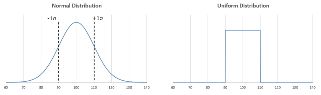
First, with the normal distribution, as shown in the figure, it becomes a Gaussian distribution centered around 100. Setting the tolerance range (v) to ±10% results in a normal distribution with a standard deviation (σ) of 10Ω. It should be noted that distributions also occur outside the range of 90~110Ω, meaning the variation range is not exactly ±10%.
For uniform distribution, it is simple with ±10%, meaning data is evenly distributed from 90 to 110Ω, and there is no data outside this range. This means the upper and lower bounds of variation are within the 10% range. However, because the ratio of the center of the data range to the upper and lower limits is equal, it is not suitable for verifying the variation ratio of actual components. Actual electronic components have the most distribution near the center of the range, with fewer variations towards the upper and lower limits, forming a normal distribution.
Important Considerations for Setting
In reality, variations of components like resistors and capacitors are normal distributions, not uniform distributions. As mentioned earlier, directly using the component’s deviation (%) as the tolerance range (v) does not allow for accurate simulation. Methods to simulate the distribution of actual components will be introduced in another article.
Conclusion
By using the tol function, you can effectively simulate random variations of input variables in Monte Carlo simulation. Understanding and properly setting the characteristics of normal and uniform distributions allows for high-precision evaluation of system performance and reliability.


Comment