How to Extract Equivalent Circuit Parameters of MLCC Chip Capacitors with uSimmics (formerly QucsStudio) [2026]

uSimmics (formerly QucsStudio) enables the extraction of equivalent circuit parameters of MLCC (Multi-Layer Ceramic Capacitors) from measured S-parameter data. This article explains how to model the non-ideal behavior of chip capacitors using vector network analyzer data, enabling high-accuracy circuit simulation.

What You’ll Learn

The difference between ideal capacitors and real MLCCs, and the effect of parasitic elements
S-parameter measurement with a VNA and data acquisition in Touchstone format
Importing and simulating S-parameters in uSimmics (formerly QucsStudio)
Building an equivalent circuit (C, L, R) and extracting parameters step by step
Optimizing inductance and resistance values using the Tune function

1. Ideal vs. Real MLCC Capacitors

Ideal Capacitor Characteristics

An ideal capacitor is defined solely by its capacitance value C. Its impedance is expressed as:

Z = 1 / (jωC) = 1 / (j × 2πf × C)

As frequency f increases, impedance decreases, attenuating high-frequency signals.

Parasitic Elements in Real MLCCs

Real MLCCs (Multi-Layer Ceramic Capacitors) contain the following parasitic elements in addition to the ideal capacitance:

Parasitic Element	Symbol	Cause	Effect
Equivalent Series Inductance	ESL (L)	Inductive structure of internal electrodes and terminals	Acts as an inductor above self-resonant frequency (SRF)
Equivalent Series Resistance	ESR (R)	Dielectric loss and electrode resistance	Increased loss at resonance, reduced Q factor

Due to these parasitic elements, real MLCCs have a Self-Resonant Frequency (SRF). Below the SRF they behave as capacitors; above it, as inductors.

SRF Calculation

SRF = 1 / (2π × √(L × C))

Above the SRF, capacitor function degrades significantly. Always verify the SRF when selecting components for decoupling and RF filter applications.

2. Significance of Equivalent Circuit Parameter Extraction

MLCC datasheets typically list capacitance C, ESL, and ESR. However, actual characteristics may differ from datasheet values depending on mounting conditions (PCB, land pattern, surrounding components).

By extracting and modeling parameters from measured S-parameters, you can achieve:

High-accuracy simulation reflecting actual mounting conditions
Precise prediction of filter and decoupling circuit characteristics
Evaluation of lot-to-lot variation in production components

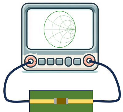
3. S-Parameter Measurement

Component Used

This article uses the following component:

Item	Specification
Component type	MLCC (Multi-Layer Ceramic Capacitor)
Capacitance	100 pF
Size	0.6 mm × 0.3 mm (0201 inch standard)

Step 1: S-Parameter Measurement with VNA

Use a Vector Network Analyzer (VNA) to measure the capacitor’s S-parameters:

Mount the MLCC on a measurement fixture
Calibrate the VNA (apply SOLT or equivalent calibration) to ensure measurement accuracy
Measure S12 (or S21) characteristics over 100 MHz to 3 GHz
Export measurement data in Touchstone format (.s2p file)

Touchstone format is the standard file format for describing S-parameters of RF devices and is supported by uSimmics (formerly QucsStudio).

4. Simulation Procedure in uSimmics (formerly QucsStudio)

Step 2: Create Circuit and Import S-Parameters

Launch uSimmics (formerly QucsStudio) and create a new schematic
Place an S-parameter file component (SPfile) from the “system components” library
Load the measured Touchstone file (.s2p) into the SPfile component
Connect signal ports and GND, creating a circuit topology with the component in shunt to GND

Step 3: Run S-Parameter Simulation and Observe Results

Place an S-parameter simulation component
Set the frequency range from 100 MHz to 3 GHz
Run the simulation and display S21 (transmission characteristic)

Observed capacitor behavior:

100 MHz to ~1 GHz: Insertion loss increases with frequency (normal capacitor operation)
Near SRF: Loss reaches maximum (series resonance minimizes impedance; maximum signal flows to GND)
Above SRF: Loss begins to decrease (inductor behavior; capacitor function degrades)

5. Building the Equivalent Circuit and Extracting Parameters

Step 4: Create the Equivalent Circuit

Build the following equivalent circuit to model the real capacitor:

Port1 ─── L1 ─── C1 ─── Port2
                  │
                GND

Element	Role	Component in uSimmics
C1 (Capacitor)	Primary capacitance	Capacitor component (with ESR input)
L1 (Inductor)	ESL (Equivalent Series Inductance)	Inductor component
R (Series Resistance)	ESR (Equivalent Series Resistance)	Series resistance property of L1

Place a Capacitor component and set C = 100 pF
Connect an Inductor component in series
Overlay the measured and simulated S-parameter results on the same graph

Step 5: Optimize Inductance Using the Tune Function

Use uSimmics (formerly QucsStudio)’s Tune function to adjust the inductance value:

Select “Simulation” → “Tune” from the menu
Select inductor L1 as the parameter to tune
Adjust the slider to find where the simulated SRF matches the measured SRF
Record the L1 value at the matching point

For the 100 pF MLCC in this example, L1 = 0.2739 nH matched the measured resonant frequency.

Step 6: Optimize Equivalent Series Resistance (ESR)

Next, adjust ESR to match the loss at resonance (depth of the S21 dip):

Open the L1 component properties and enter the initial ESR value under Series Resistance
Typical chip capacitor ESR is 0.1 Ω to 0.2 Ω — use this as a starting point
Use the Tune function to adjust ESR until the simulated resonance dip matches the measured data
For this component, ESR = 0.18 Ω provided a good match

6. Summary of Extracted Parameters

Extracted equivalent circuit parameters for the 100 pF MLCC in this article:

Parameter	Symbol	Extracted Value
Capacitance	C	100 pF (nominal)
Equivalent Series Inductance	ESL (L)	0.2739 nH
Equivalent Series Resistance	ESR (R)	0.18 Ω
Self-Resonant Frequency	SRF	≈ 963 MHz

Using this equivalent circuit model enables high-accuracy simulation of circuits containing 100 pF MLCCs.

7. Applications of the Equivalent Circuit Model

The extracted parameters can be applied to the following design and simulation scenarios:

Decoupling circuit design: Optimal capacitance and size selection considering SRF for power line decoupling
LC filter design: Accurate prediction of passband and stopband characteristics
RF matching circuit design: High-accuracy simulation of matching circuits containing chip capacitors
EMC analysis: Analysis of EMI propagation paths using equivalent circuits with parasitic elements

8. Conclusion

By leveraging the Tune function in uSimmics (formerly QucsStudio), you can accurately extract MLCC equivalent circuit parameters (C, ESL, ESR) by iteratively comparing measured and simulated S-parameters. Integrating the extracted parameters into an equivalent circuit model enables high-accuracy simulation that reflects actual mounting conditions, improving circuit design reliability and quality.