
In the previous article, we explained the basics of using the “tol” function. This time, we will dive deeper into the detailed settings and customization of the “tol” function. Specifically, we will explain the adjustment of standard deviation and how to simulate the actual distribution of components.

Standard Deviation Settings Based on Actual Component Distribution
In Monte Carlo analysis, it is essential to accurately reproduce the variation of components. As mentioned in the previous article, the manufacturing variation of components typically follows a normal distribution. Manufacturers manage these variations to ensure that they fall within a specific range as part of quality control.
Resistors with a general ±5% tolerance are managed in the manufacturing process so that this range corresponds to 3σ (3 sigma). This ensures that 99.73% of the manufactured resistors fall within this ±5% range, reducing the occurrence of defective products. In this case, 1σ is equivalent to 1/3 of the tolerance range.
Why Is the Tolerance 3σ and Not 1σ?
In manufacturing, the “3σ (3 sigma)” standard is commonly used for quality control. Here, 3σ refers to the range within which 99.73% of the data in a normal distribution falls, with three standard deviations from the mean. This method is used to minimize defective products.
For example, if a resistor has a nominal value of 100Ω and a tolerance of ±5% (95Ω to 105Ω), manufacturers ensure that 99.73% of the products are within this range. This means that the ±5% range corresponds to 3σ.
Difference Between 1σ and 3σ
1σ (1 sigma) is the range within one standard deviation from the mean, covering about 68.27% of the data in a normal distribution. If the tolerance were set to 1σ, the chance that the product’s characteristics would fall within ±1σ would be only 68.27%. In contrast, with 3σ, the data is much more tightly clustered within the range, covering 99.73%.
Using the 3σ standard ensures that most products stay within the expected range, which is crucial for quality control. By using a 3σ tolerance, the percentage of defective products is kept very low.
Detailed Explanation
Let’s take a 100Ω resistor as an example. With a tolerance of ±5%, the resistor’s actual value should fall within the range of 95Ω to 105Ω.
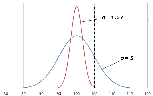
3σ Setting: Manufacturers set the process so that the product falls within the range of 95Ω to 105Ω (±5%) with a probability of 99.73%. This means the ±5% range corresponds to 3σ. Therefore, 1σ is one-third of this range, which equals 1.67Ω.
1σ Calculation: Since the ±5% range corresponds to 3σ, 1σ is one-third of that. For a 100Ω resistor, 1σ would be approximately 1.67Ω (5Ω ÷ 3 ≈ 1.67Ω).
Thus, when a manufacturing process is managed based on the 3σ standard, the tolerance range (±5%) covers 99.73% of the products. This setting ensures product reliability and quality, reducing the defect rate to less than 0.27%.
Specific Simulation Settings
Let’s continue with the example of a 100Ω resistor. If the manufacturing error is ±5%, the resistor’s value should fall within the range of 95Ω to 105Ω. Assuming this range represents 3σ, the standard deviation for 1σ can be calculated as follows:
σ = (100 × 0.05) / 3 ≈ 1.67 Ω
By using this 1σ value, you can set the “tol” function to simulate the actual component distribution more accurately.
Example of “tol” Function Setting
In QucsStudio, to reflect this standard deviation in the simulation, you can set the “tol” function as follows:
tol(100, 1.67, 0)
Here, 100 is the target resistor value (mean), 1.67 is the standard deviation (tolerance), and 0 indicates a normal distribution. This setting allows Monte Carlo analysis to simulate the component variation based on actual manufacturing processes.
Significance and Effect of the Settings
By accurately setting the standard deviation, the simulation results will show that 99.73% of the resistor values fall within the range of 95Ω to 105Ω. This closely matches the actual component distribution in the manufacturing process. As a result, designers can evaluate circuit performance more precisely in real-world manufacturing environments.
Simulations that consider component variation not only enhance the reliability of the design but also contribute to better quality control in production.
📌 See the recommended reading order (Roadmap)
➡️ Next: Parametric analysis (comparison)

Comment